I appreciate birds (but not enough to birdwatch) and funky Neural Network achitectures that aren’t a product of mixing a bunch of functions in a pot and optimizing hyperparameters. Ian Goodfellow’s paper was my first exposure to Generative Adversarial Networks and their beautiful architecture. I’ve wanted to try training one for a while now, but was hardware-limited and unwilling to spend the beacoup bucks on a Colab or AWS instance. I built a PC in early January, straddling the line nicely enough between frugality and beefiness to make training a GAN worthwile (still took 8 hours every day for a week though!).
I’ve always been fascinated with old zoology illustrations, and how they used to border on the fantastical. Birds are diverse enough that I thought I’d get some pretty results out of a network trying to generate the diversity in our avian friends’ plumage, beaks, size and everything in between.
Training progress:
How do GANs work?
Generative models take a training set, consisting of samples drawn from a distribution $ p_{data} $ and learn to represent an estimate of the distribution $ p_{model} $. This is the fundamental basis behind all generative models. GANs work by gamifying the task between two functions, a generator and a discriminator. The generator, represented by a function $G(x)$ seeks to generate samples to fool the discriminator, $D(x)$ which for simplicity’s sake is a traditional supervised learning classifier. Given parameters for each function, ($ \theta^{(G)} $) and ($ \theta^{(D)} $ respectively), both functions seek to minimize their cost functions ($ J $) while only controlling their parameter:
$$ J^{(D)}(\theta^{(D)}, \theta^{(G)}) $$
Since each function can only influence their own parameters, the solution to this optimization problem is a Nash Equilibrium (as the solution is a local minimum where all neighboring points have higher cost). There are several possible cost functions that can be used, but they’re out of the scope of this post and a good explanation to them can be found here.
The StyleGAN/2 Architecture
StyleGAN is a novel architecture in the GAN space, which borrows from style transfer - representing image 1 with the style of image 2. StyleGAN aimed to address the black-box nature of most GAN models, where insight into the model’s latent space were lacking. The latent space of any neural network is the compressed feature space. As a model learns, data dimensionality decreases, and all relevant information needs to be compressed while noise is discarded. Think about the density of information contained in the components of a phone and the level of information used to identify a phone as a phone to us.
Before StyleGAN, few GANs could distinguish which parts of the latent feature space corresponded to image features (i.e human face generation -> hair color, eye color, etc). I’m going to try and explain what StyleGAN does as best I can, but highly recommend reading the paper. Don’t be fooled by the names like AdaIN, PixelNorm or Conv, just think of them as matrix transforms of data. The core of most ML is really just a series of matrix transforms applied (sometimes seemingly randomly). Below is the generator architecture (from the paper):
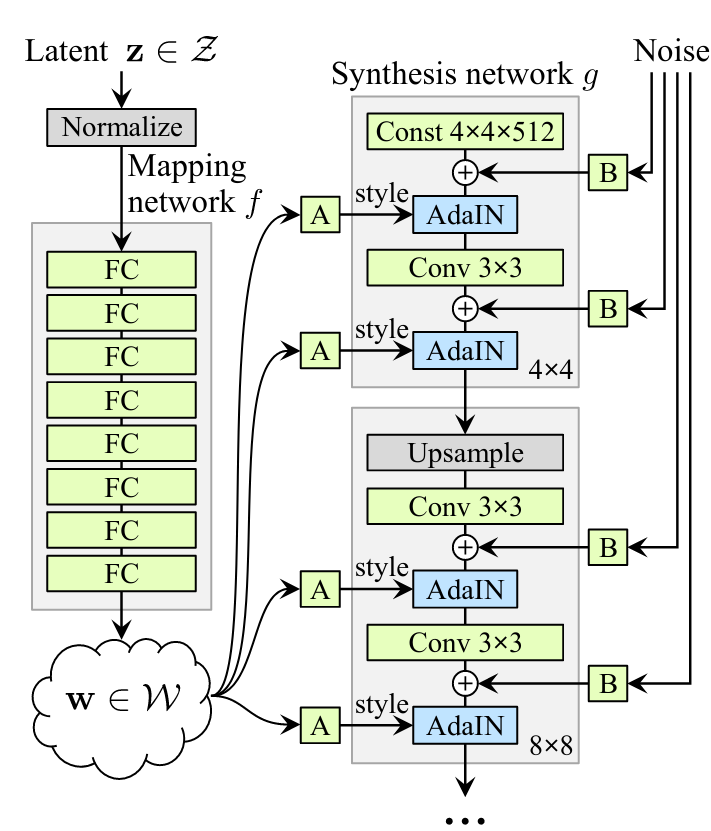
Let’s break it down.
AdaIN & Conv
AdaIN == Adaptive Instance Normalization. The operation is defined as: $$ \text{AdaIN}(\vec{x_{i}}, \vec{y}) = \vec{y_{s,i}} \frac{\vec{x_{i}} - \mu (\vec{x_{i}})}{\sigma \vec{x_{i}}} + \vec{y_{b, i}} $$
$\vec{x_{i}}$ are feature maps generated from the convolution layers - activation matrices generated through feature detection. The feature maps are normalized and biased with components from the style $\vec{y}$. This is how the style transfer works, $y$ is the style input, and $x$ is a feature map. Think about style transfer as applying Van Gogh’s signature style to a picture of a cityscape.
Affine Transforms, Noise and Progressive Growth
A and B correspond to learned affine transforms and gaussian noise respectively. An affine transform is a linear matrix transformation that preserves lines and parallelisms. The affine transformations are used to specialize $\vec{w}$ from the intermediate latent space. The output of each Conv layer is a block of activation maps. Noise is added to each of these maps, used to introduce variation in the generated images.
Progressive growth here involves slowly growing the model, starting at 4x4 and moving up progressively to the target dimensions. Upsampling is performed with nearest neighbor layers to grow the model.
Dataset
I sourced the dataset from the Biodiversity Heritage Library’s Flickr feed which is well worth browsing and also following on twitter. I went after albums that were already ornithology focused to minimize data munging. The images were understandably different resolutions, so a quick and dirty python script to make the image square and then resize to 512x512 was needed:
import os
import glob
import uuid

from PIL import Image

# lop off the top of the image to make it square, then resize to 512, 512
def lop_off(pil_img):
    img_width, img_height = pil_img.size
    crop_start = abs(img_height - img_width)/2

    (left, upper, right, lower) = (0, crop_start, img_width, (img_height-crop_start))

    cropped_img = pil_img.crop((left, upper, right, lower))
    resized_img = cropped_img.resize((512, 512))
    return resized_img

def main(raw_dir, save_dir):
    # loop through
    for img in glob.glob(raw_dir+'/*.jpg'):
        image = Image.open(img)
        filename = "".join(sample(digits, 10))+'.jpg'

        resized_img = lop_off(image)
        resized_img.save(save_dir+'/'+filename)
StyleGAN2 requires that the images be converted to TFRecords, a tensorflow specific filetype. This is easily done with one of the utility scripts provided in the repo.
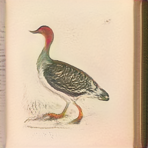
For reference, this is what one of the training images looked like:
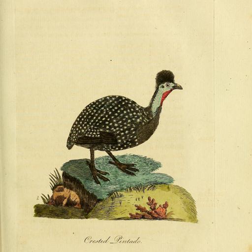
I intentionally didn’t clean up the images by removing text, normalizing the background or removing borders. I wanted to see how StyleGAN2 would deal with those kinds of details in the latent space and how they’d be incorporated while interpolating on the space to generate images.
Training
Training took a total of ~40 hours, trained using 2000 kimg (2 million images) on an Nvidia 2070 Super w/ 8G of VRAM. It’s clear the authors trained their models in one go, because there wasn’t a readily accessible way of resuming training from a checkpoint. I had to scrape around the code a little - a modified StyleGAN2 codebase is available w/ incredibly simple instructions on how to resume training on my github here.
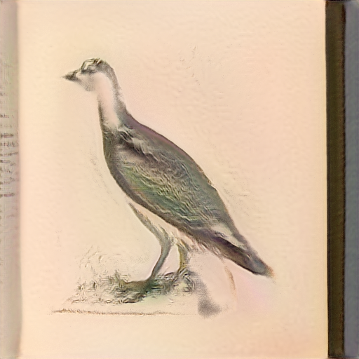
Results
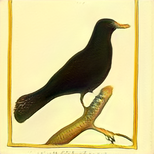
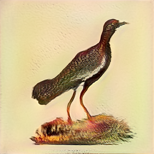
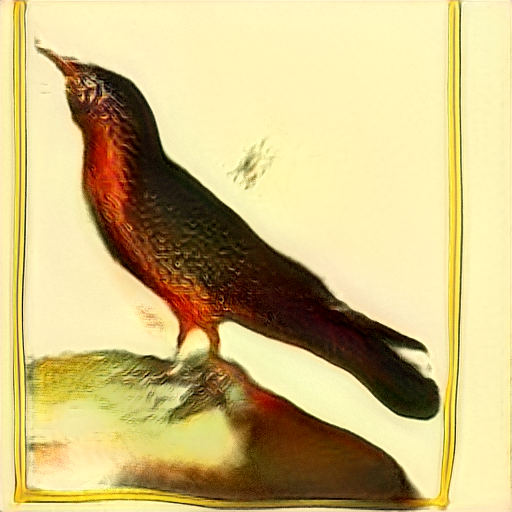
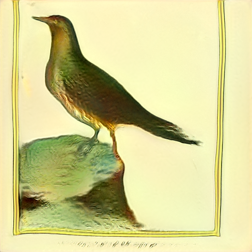
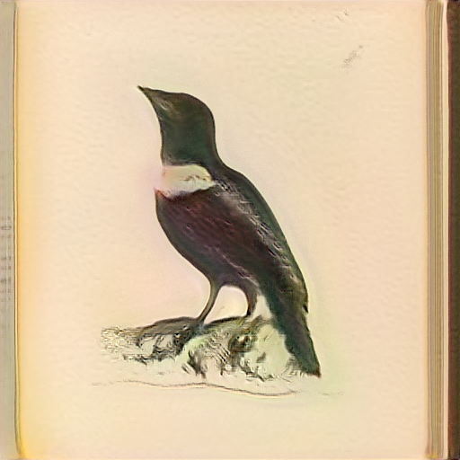
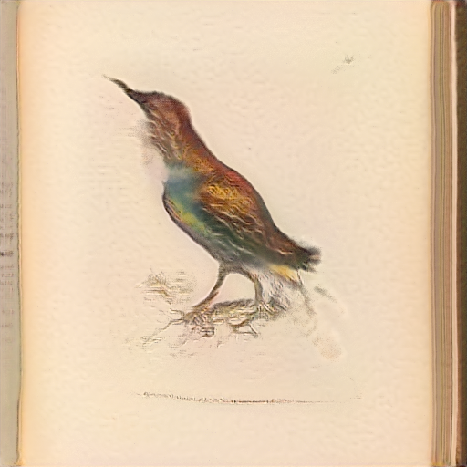
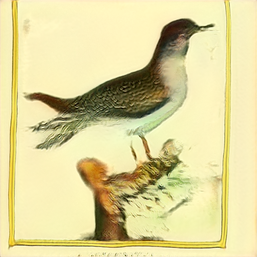
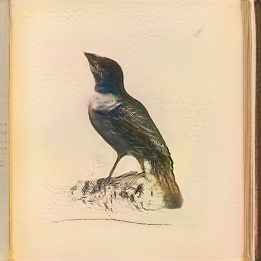
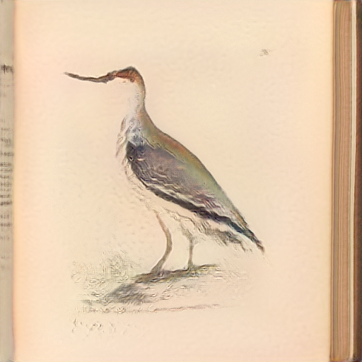
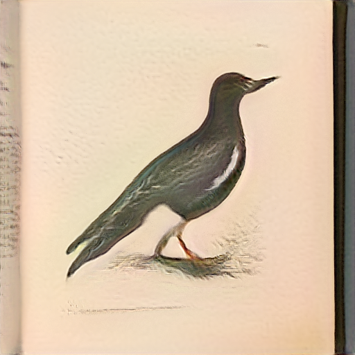
Below are images generated from seeds I’ve selected that look the best. These birds do not exist!
This was fun, but I’m not likely to go through personally training a large model from scratch again. I had to restart training multiple times to play around with the config, throwing away days of generated models. This ties in with how I feel right about the state of ML/AI right now and the use of compute resources. I personally find the efforts of ML researchers working with underpowered hardware to be a lot more inspired because I believe that constraints make for more creative problem solving. See for example what it took to train GPT-3. This is not to say that the work that OpenAI did on GPT-3 or Nvidia on StyleGAN is not worth it - the insight we gain from their research has led to major gains in ML. I’ve just come to realize that training a large model isn’t fun for me. I have a couple ideas that aim to buck the trend of the massive models that I’m now super excited to try out and write about. I’ve put a couple links that are helping me form these ideas in the section below.
In some personal news, I’ve gone fully remote now, and am moving to NYC in August. I’ll hopefully have a lot more time to write about some of the projects I’m working on.