I’ve been working on and off on the Planetary Defence Challenge, a competition hosted by ESA. I’ll explain the basic premise below, and if you want more details on the details, check out the link.
The ESA has been working on a kinetic impactor mission as part of an effort to prepare for the need to deflect an asteroid. The actual effects of an impact are highly dependent on many factors, but the one most pertinent to this problem is the $ \beta $ factor, which is the ratio of linear momentum actually transferred to a body post collision vs. linear momentum transferred in the case of a perfectly plastic collision.
The specific scenario being observed is a binary system, with a primary asteroid orbited by a secondary:
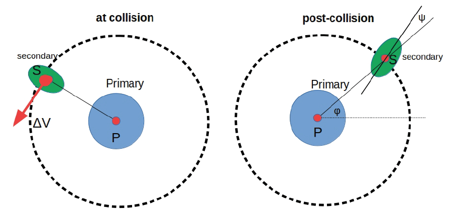
The catch here is that the only data that we’ve got are lightcurves from the system - light intensity as functions of time. Intuitively, dips in intensity correspond to when the orbiting body passes in front of the primary body. This is all we have to go on though, and where things can get interesting. The problem is “solved” if we can predict the $\beta$ factor, $J2$ (the spherical harmonic coefficient of the primary body), and $a/c$, the ratio of the semimajor and semiminor axes of the secondary body (the one that’s getting deflected).
In essence, the problem boils down to:
Given sparse lightcurve data before and after collision, is it possible to extract or estimate parameters that describe the system and dynamics?
Baseline Approach
Trying to embed or use any physical information about the system didn’t get me very far. Extracting information from lightcurves is an open problem, and I got stuck early trying to derive orbital parameters from lightcurve data. It’s still possible, but at the time I was time constrained and wanted a quicker solution.
I ran out the clock on the problem, freeing me up to pursue flights of fancy that are less brute-forcey (more details on this in a bit). Part 1 of this series is really about how I set up the problem using Julia and how I developed a fairly generic way of starting to apply machine learning to problems like this.
If you’ve heard me rant/rave about ML, you already know a pretty big pet peeve is its needless application (e.g in places where a purely analytical solution is much faster (albeit less sexier)). There is no good analytical solution to this problem (I think, also more on this later), which is why it still interests me.
Julia & ML
I’ve been using Julia a lot this year, and find myself reaching for it now over Python or Matlab. I’m not going to soapbox on why I enjoy using it so much more, there are hundreds of articles floating around already that do a much better job than I could hope to. The key player here is Flux, an ML framework written in pure Julia. It’s got some pretty neat abstractions that make iterating on a problem really really fast, much faster than if I were to use Tensorflow.
The light curves needed data munging, since they cover slightly different periods. This was an easy enough problem to solve by just interpolating the data to a fixed timescale. Input size needs to be consistent across data if you’re throwing it into the proverbial ML pot. After that, it’s really as simple as:
function train_barebones!(hyper_params::TrainingParams)
    model = Chain(
        Dense(84, 21, relu),
        Dense(21, 7, relu),
        Dense(7, 2))
    # given a before and after lightcurves. Can we encode data in the difference b/ween them?
    before, after = Utils.interpolate(1, 100)

    opt = Descent(hyper_params.learning_rate)
    loss(x, y) = Flux.Losses.msle(model(x), y)
    pm = params(model)
    epochs = hyper_params.epochs

    epoch_loss = zeros(epochs)
    for epoch in 1:epochs
        interm_loss = zeros(100)

        for sample in 1:100
            y_train = Utils.munge_training_data(sample)
            x_train = before[:, 2, sample] - after[:, 2, sample]
            data = [(x_train, collect(y_train))]

            train!(loss, pm, data, opt)

            interm_loss[sample] = loss(x_train, y_train)
            @show(interm_loss[sample])
        end

        @show(params(model))
        epoch_loss[epoch] = mean(interm_loss)
    end

    weights = params(model)

    @save "barebones.bson" weights
end
The model here is a Chain of different layers, followed by an activation function. That’s it. My model is 3 layers, an input layer w/ dimensions 84x21 (84 time samples, 21 potential features in the data), a hidden layer w/ dimensions 21x7 and an output layer of size 7x2. The 1x2 vector output we want at the end holds $\beta$ and $ a/c $.
After that, it’s just iterating over data and validating with a loss function. train!is doing a lot of the heavy lifting here, performing the gradient descent and updating model weights as the loss is evaluated (! means its a function that mutates things you pass to it).
This super simple approach gets me much further on the leaderboard than I thought it would (list goes on further).
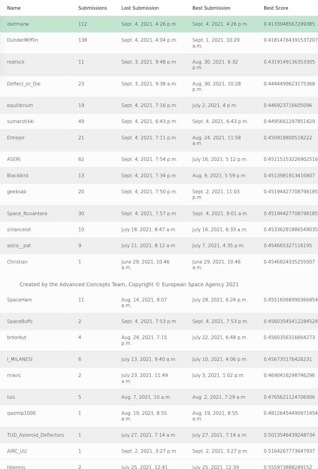
For reference, the score here is evaluating the $\beta$ and $a/c$ that you generate and plugging it into a function. As an aside, the function itself was apparently slightly flawed, and I was a little higher on the leaderboard before it demoted me.
Take a look at the scores and # of submissions. After ~0.46, it starts becoming a crapshoot, and the fight is for a better score on the order of a few decimal places. Training a model is decidedly non-deterministic - you’re not guaranteed the same output unless you’re using the exact same set of weights.
Getting to the top is then a matter of iterating many, many times, performing some kind of hyperparameter or model optimization, and crossing your fingers.
I started down this path before the tediousness caught up to me - my interest in the problem is first and foremost applying ML to a dynamic system in space. With this in mind, I’ve started exploring some other avenues which I’ll briefly touch upon here, and expand in Part 2, once I’ve worked on them a little more and have something to show for it.
Funner stuff
Angular Velocity, Glint and Light curves
My model was ingesting everything in the data. The hidden layer size is large enough for there to possibly be some representation of features inherent in the raw data, but there’s no guarantee of it. I read a few papers before finding specular glint, which Dr. Crassidis uses in this paper to develop angular velocity bounds for an object that’s being observed (and subsequently generating light curves). In short, glint is a feature of the light curve data that corresponds to peaks in the curves.
I’ll address ways of getting glint and the angular velocity in Part 2.
Koopman Operators & SINDy Autoencoders
Any explanation I give won’t do the Koopman operator justice, so I’ll give a very bird’s eye view of it. In short, it’s a method to represent a non-linear function or dynamic system linearly. Specifically, the main idea is to find an approximated linear representation, and then use it to obtain an exact solution. SINDy here stands for Sparse Identification of Nonlinear Dynamics. Bird’s eye view again: if we reduce/minimize a dataset to the barest features that you can use to represent the system, you’re very very close to learning the governing equations that describe the system.
It sounds deceptively simple, but there’s a lot going on behind the scenes that I don’t really fully understand. I’ll leave a better explanation to part 2. I’m using this incredible video as reference: Deep Learning to Discover Coordinates for Dynamics: Autoencoders & Physics Informed Machine Learning. Incredibly, it hits every buzzword that I’m interested in and tingles all the right parts of my brain. Koopman + Autoencoders is what I’m currently trying to apply to the problem, so stick around for updates on that. Check out this paper for more info.